Euler-Heisenberg Lagrangian

In physics, the Euler-Heisenberg Lagrangian describes the non-linear dynamics of electromagnetic fields in vacuum. It takes into account vacuum polarization to one loop, and it is valid for electromagnetic fields that change slowly compared to the inverse electron mass. It was first obtained by Werner Heisenberg and Hans Heinrich Euler,^[1] and can be expressed as:

$\mathcal{L} =-\mathcal{F} -\frac{1}{8\pi^{2}}\int_{0}^{\infty}\frac{ds}{s^{3}}\exp\left(-m^{2}s\right)\left[(es)^{2}\frac{\operatorname{Re}\cosh\left(es\sqrt{2\left(\mathcal{F} %2B i\mathcal{G}\right)}\right)}{\operatorname{Im}\cosh\left(es\sqrt{2\left(\mathcal{F} %2B i\mathcal{G}\right)}\right)}\mathcal{G}-\frac{2}{3}(es)^{2}\mathcal{F} - 1\right]$

Here m is the electron mass, e the electron charge,

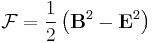
$\mathcal{F}=\frac{1}{2}\left(\mathbf{B}^2 - \mathbf{E}^2\right)$ ,

and

$\mathcal{G}=\mathbf{E}\cdot\mathbf{B}$

In the weak field limit, this becomes:

$\mathcal{L} = \frac{1}{2}\left(\mathbf{E}^{2}-\mathbf{B}^{2}\right)%2B\frac{2\alpha^{2}}{45 m^{4}}\left[\left(\mathbf{E}^2 - \mathbf{B}^2\right)^{2} %2B 7 \left(\mathbf{E}\cdot\mathbf{B}\right)^{2}\right]$

References

^ W. Heisenberg and H. Euler,Folgerungen aus der Diracschen Theorie des Positrons Z. Phys. 98, 714 (1936).